
Technical Tutoring Home · Site Index · Advanced Books · Speed Arithmetic · Math Index · Algebra Index · Calculus Index · Trig Index · Chemistry Index · Gift Shop · Harry Potter DVDs, Videos, Books, Audio CDs and Cassettes · Lord of the Rings DVDs, Videos, Books, Audio CDs and Cassettes · Winnie-the-Pooh DVDs, Videos, Books, Audio CDs, Audio Cassettes and Toys · STAR WARS DVDs and VHS Videos
Construction of the Riemann Integral
Introduction · Definition of the integral · Examples · Conclusion · Recommended Books
The "inverse" operation of differentiation is integration. Geometrically, we use the derivative of a function to get the slope of the function at a given point. We use the integral of a function to get the area under the curve:
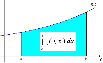
Figure 1 - The definite integral of f(x) between "a" and "b"
Let’s take a closer look at the symbol that represents the integral.

The elongated "S" stands for integral. Clearly, f(x) is the function being integrated. The two numbers "a" and "b" are the lower and upper limits of the integral – we need these to define where the area under the curve starts and ends. Finally, the symbol "dx" tells us we are integrating with respect to x.
The integral above is a number, rather than a function. Given a definite, legal (integrable, see below) function and definite, legal limits, the area under the curve is well-defined and has a numerical value. Of course there are technical variations that get complicated, but we will stick to the simple case pictured above for now.
The function f(x) pictured above is a curve and so changes in value as x changes. Up to this point, the only methods for calculating area we know are for simple geometric shapes, particularly rectangles:
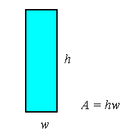
Figure 2 - Area of a rectangle = height times width
We’ll use rectangles to figure our area, even though rectangles are a bit crude. To make our area more accurate, we’ll add more rectangles as needed. This is a variation on successive approximations, a method we have used elsewhere. Boiled down, our method will be to define a crude approximation to the area we want. The crude approximation will have one very important property – it can be refined. We’ll make better and better refinements to the area (by adding more rectangles) until we have something we can use in a limit. Adding the limiting process is what makes this calculus.
The crudest approximation we can make is to use one rectangle. We have two choices for the height of the rectangle, the minimum value of f(x) for x in [a, b] and the maximum value of f(x) for x in [a, b]:
If we choose the minimum value for f(x), in this particular case, f(a), we’ll get a rectangle that looks like this:
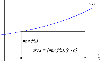
Figure 3 - First approximation of integral using minimum value of f(x)
As mentioned above, the height of the rectangle is chosen as the minumum value of f(x) for x in [a, b], in this case that happens to be h = f(a). The width of the rectangle is the difference between the endpoints, w = b – a. In this case, the area approximation is
![]()
This notation means that A is the area approximation, underlined to emphasize we are approximating the area from below (so that the approximation is less than the "real" area), and depends on two quantities, f(x), the function, and P, the partiiton or way we have sliced up the interval [a, b]. This is the first approximation and so P is just the interval [a, b]. Note well that the value of this approximation, f(a)(b – a), is well-defined. If we know f(x), "a" and "b", we can actually calculate this number.
Suppose instead we use the maximum value of f(x) over the interval as the height of the rectangle. The rectangle looks like this:
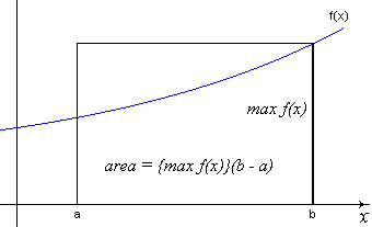
Figure 4 – First approximation of integral using maximum value of f(x)
Our approximation in this case becomes:
![]()
This notation means that our area approximation, overlined to emphasize that this estimate overshoots the "real" area, is found from the maximum of f(x) and the width of the interval. Again, the value of the approximation, f(b)(b – a), is easy to calculate explicitly if f(x), "a" and "b" are known.
Although it is obvious from statements above, we should still point out that
![]()
This fact will still be true in the development below. All it says is that our estimates always undershoot and overshoot the "real" area, respectively.
To get a better estimate, we take a second approximation. Refining the estimate is simply a matter of changing the partition. The first partition was simply
![]()
To improve the estimate, we cut this interval into two equal pieces:
![]()
Note that x0 = a and x2 = b. Most math texts will simplify this notation to
![]()
The understanding is we have an interval between each pair of successive x’s. We will use this simplification as well, but the reader should think of the list of x’s as the endpoints of a list of intervals, similar to the far right-hand side of the definition of P in the next to last equation above.
Our two area estimates now look like:
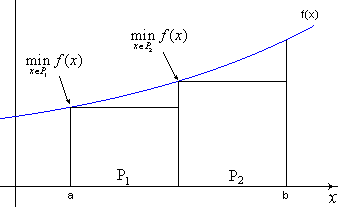
Figure 5 - Second approximation using minimum values of f(x)
and
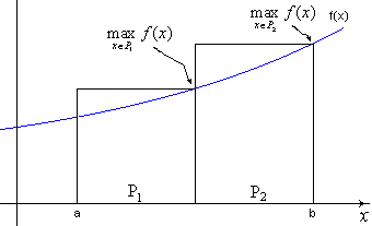
Figure 6 - Second approximation using maximum values of f(x)
Now we have
![]()
and
![]()
The "real" area, in other words, the integral, is still between these two estimates.
As a brief aside, the reader might have noticed that the notation to express these estimates is getting rather intricate and difficult to read. In the subsequent development, we will again alter our notation a bit to improve the readability; however, the basic process has been established. We will refine our estimates by chopping up the interval [a, b] into ever-smaller pieces and calculate the upper and lower estimates each time.
Suppose we have done this several more times, in fact, n times. Now, each piece of the interval has the same width:
![]()
The function f(x) we have shown in the graphs is increasing, so the minimum for each piece is at the far left end of the piece while the maximum is at the far right end. We want our development to be true regardless of how f(x) behaves over [a, b], so we won’t use this particular specific fact about our example function. Instead, we will give our maximums and minimums of f(x) in each piece a special name. Set

Now, our rectangles look something like this:
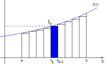
Figure 7 - nth approximation using minimum values of f(x)
and
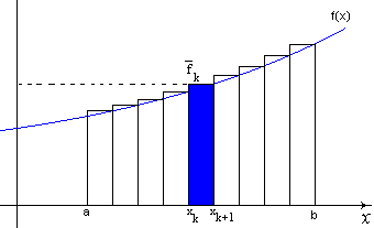
Figure 8 - nth approximation using maximum values of f(x)
As before, we will add up the area from each rectangle created from each piece. For each piece, we have the lower and upper estimates of the area under f(x)

Adding the pieces gives
![]()
as the lower estimate and
![]()
as the upper estimate. In both cases, we were able to move the width of the interval, Dx, outside the summation symbol because all the pieces have exactly the same width and are independent of the index k. In fact, we can change our notation again to reflect the fact that our estimates actually depend on the number of rectangles (pieces), n:
![]()
![]()
Here we substitued the previously discussed formula for the width of the intervals.
Thus far, no use of calculus (ie limiting processes) has been made. Now we are in a position to make use of limits to drive our estimates automatically. For the lower estimate, we’ll define a number called the lower integral as
![]()
Similarly, we define the upper integral as

Analogously with our previous statements about the upper and lower estimates above, we have

In the happy case where we have

the function f(x) is said to be integrable and both the upper and lower integrals are equal to the integral

Examples Integral of a constant · Calculation of the integral of the function f(x) = x · Calculation of the integral of the function f(x) = x2
Example - Integral of a constant
Find the area under the constant function f(x) = 1 from a = 2 to b = 4.
Solution
We need the following sum
![]()
Since this function is constant, f(x) = 1 everywhere, and there is no need to worry about lower and upper integrals. We’ll use the formula for the lower integral since it looks a little easier to use:

Note that once the n was canceled from the numerator and denominator, what was left (2) did not depend on n, so we simply dropped the limit.
Example - Calculation of the integral of the function f(x) = x
Calculate
![]()
Solution
In this case,

Our strategy will be to use the estimates derived above. To do this easily, we’ll need the help of the sum:
![]()
These relations can be verified by trying the first few cases (n=1, n=2, n=3). Proof for all n is delayed until we discuss numerical sequences and series later on. Turning to the problem at hand, consider a single (sub)interval after we have chopped our interval of integration [1, 2] into n pieces:

This merely reflects the fact that the minimum of x in the interval [xk, xk+1] is xk while the maximum is xk+1. In fact, we can go further and note that
![]()
Similarly,
![]()
We now have enough information gathered to compute the lower and upper integrals.
The lower integral turns out to be

Notice that we removed the summations by use of the two formulas above. The upper integral, similarly, is found as
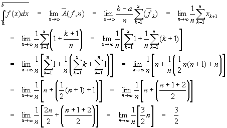
Since the upper and lower integrals are the same, the function f(x) = x is integrable over [1, 2] and its integral is 3/2.
Example - Calculation of the integral of the function f(x) = x2
Compute the integral of x2 over the interval [0, 1]. Assume that, since this function is continuous, the upper and lower integrals are identical, so it is only necessary to use, say, the lower integral. The sum
![]()
will prove helpful in the computation.
Solution
The function f(x) = x2 is an increasing function over the interval [0, 1], so we can take the minimum in each subinterval as the left-hand function value:
![]()
Substituting for xk
![]()
So that now the lower integral (by assumption, the integral) becomes

We have constructed the integral using a rather general approach and applied it to several simple examples. The alert reader will notice that using this construction to compute the integral seems to always require knowledge of sums of series. This is usually the case. Since summing series is often considered an advanced technique, the approach seen here is rarely used in typical undergraduate calculus classes. It is presented here to show the reader that the definition of the Riemann integral can indeed be used to directly compute integrals.
The method is somewhat laborious, even for simple functions, but has the advantage of always yielding the right answer (given that f(x) is integrable – we have not really covered this topic at all yet). Other, simpler techniques of calculating integrals will be shown in subsequent articles.
It should be pointed out that for numerical (ie computer) calculations of integrals, the technique shown above is very useful. Many otherwise impossible functions can be numerically integrated, allowing scientific and engineering calculations to proceed even though the functions involved have no "pure" mathematical method to find the integral. For this reason, the technique presented here should be considered important enough to commit to memory. There are tables of sums available should the need arise.
 Schaum's Outline
of Calculus (Schaum's...
 Schaum's Easy
Outline: Calculus
ã 1996 - 2002
Hyper-Ad Communications. All Rights Reserved.